Rows: 90,102
Columns: 126
$ folioviv <chr> "0100005002", "0100005003", "0100005004", "0100012002", "01…
$ foliohog <chr> "1", "1", "1", "1", "2", "1", "1", "1", "1", "1", "1", "1",…
$ ubica_geo <chr> "01001", "01001", "01001", "01001", "01001", "01001", "0100…
$ tam_loc <chr> "1", "1", "1", "1", "1", "1", "1", "1", "1", "1", "1", "1",…
$ est_socio <chr> "4", "4", "4", "3", "3", "3", "3", "4", "4", "4", "4", "3",…
$ est_dis <chr> "003", "003", "003", "002", "002", "002", "002", "003", "00…
$ upm <chr> "0000001", "0000001", "0000001", "0000002", "0000002", "000…
$ factor <dbl> 206, 206, 206, 167, 167, 167, 167, 212, 212, 212, 212, 184,…
$ clase_hog <chr> "3", "2", "2", "3", "1", "2", "2", "1", "2", "2", "2", "1",…
$ sexo_jefe <chr> "2", "1", "1", "1", "1", "1", "2", "2", "2", "1", "1", "1",…
$ edad_jefe <dbl> 91, 68, 56, 87, 27, 57, 47, 75, 70, 69, 48, 73, 64, 55, 58,…
$ educa_jefe <chr> "03", "08", "10", "11", "08", "08", "10", "06", "10", "04",…
$ tot_integ <dbl> 3, 2, 3, 4, 1, 4, 4, 1, 3, 2, 5, 1, 4, 3, 1, 6, 4, 2, 3, 1,…
$ hombres <dbl> 0, 1, 2, 2, 1, 2, 2, 0, 1, 1, 1, 1, 1, 1, 0, 1, 1, 1, 3, 0,…
$ mujeres <dbl> 3, 1, 1, 2, 0, 2, 2, 1, 2, 1, 4, 0, 3, 2, 1, 5, 3, 1, 0, 1,…
$ mayores <dbl> 3, 2, 3, 4, 1, 3, 4, 1, 3, 2, 5, 1, 4, 2, 1, 4, 4, 2, 1, 1,…
$ menores <dbl> 0, 0, 0, 0, 0, 1, 0, 0, 0, 0, 0, 0, 0, 1, 0, 2, 0, 0, 2, 0,…
$ p12_64 <dbl> 2, 1, 3, 2, 1, 3, 4, 0, 2, 0, 5, 0, 4, 2, 1, 4, 3, 0, 1, 1,…
$ p65mas <dbl> 1, 1, 0, 2, 0, 0, 0, 1, 1, 2, 0, 1, 0, 0, 0, 0, 1, 2, 0, 0,…
$ ocupados <dbl> 1, 2, 2, 0, 1, 3, 1, 0, 3, 1, 1, 0, 1, 1, 0, 3, 1, 1, 1, 1,…
$ percep_ing <dbl> 3, 2, 2, 2, 1, 4, 2, 1, 3, 2, 1, 1, 2, 2, 1, 3, 2, 2, 1, 1,…
$ perc_ocupa <dbl> 1, 2, 2, 0, 1, 3, 1, 0, 3, 1, 1, 0, 1, 1, 0, 3, 1, 1, 1, 1,…
$ ing_cor <dbl> 56123.75, 108048.87, 133852.88, 105054.15, 24211.95, 121649…
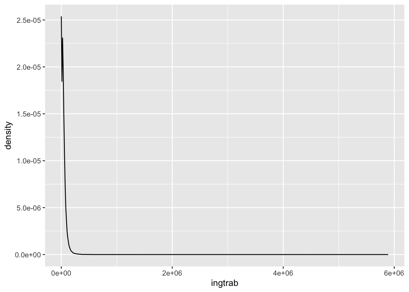
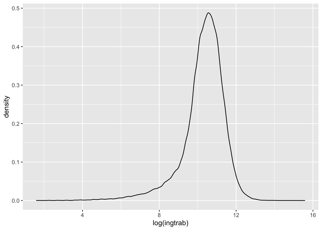
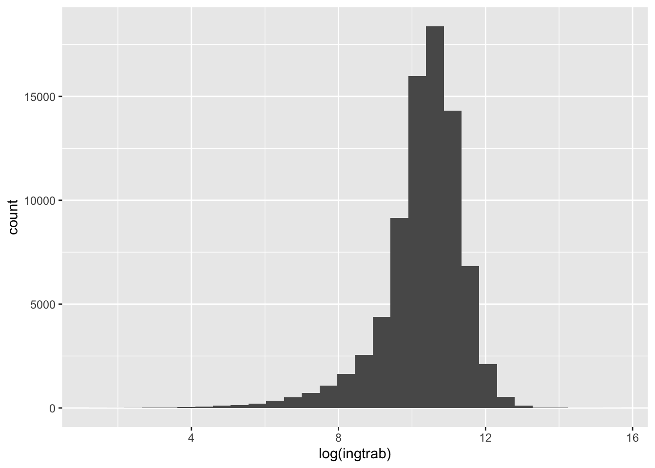
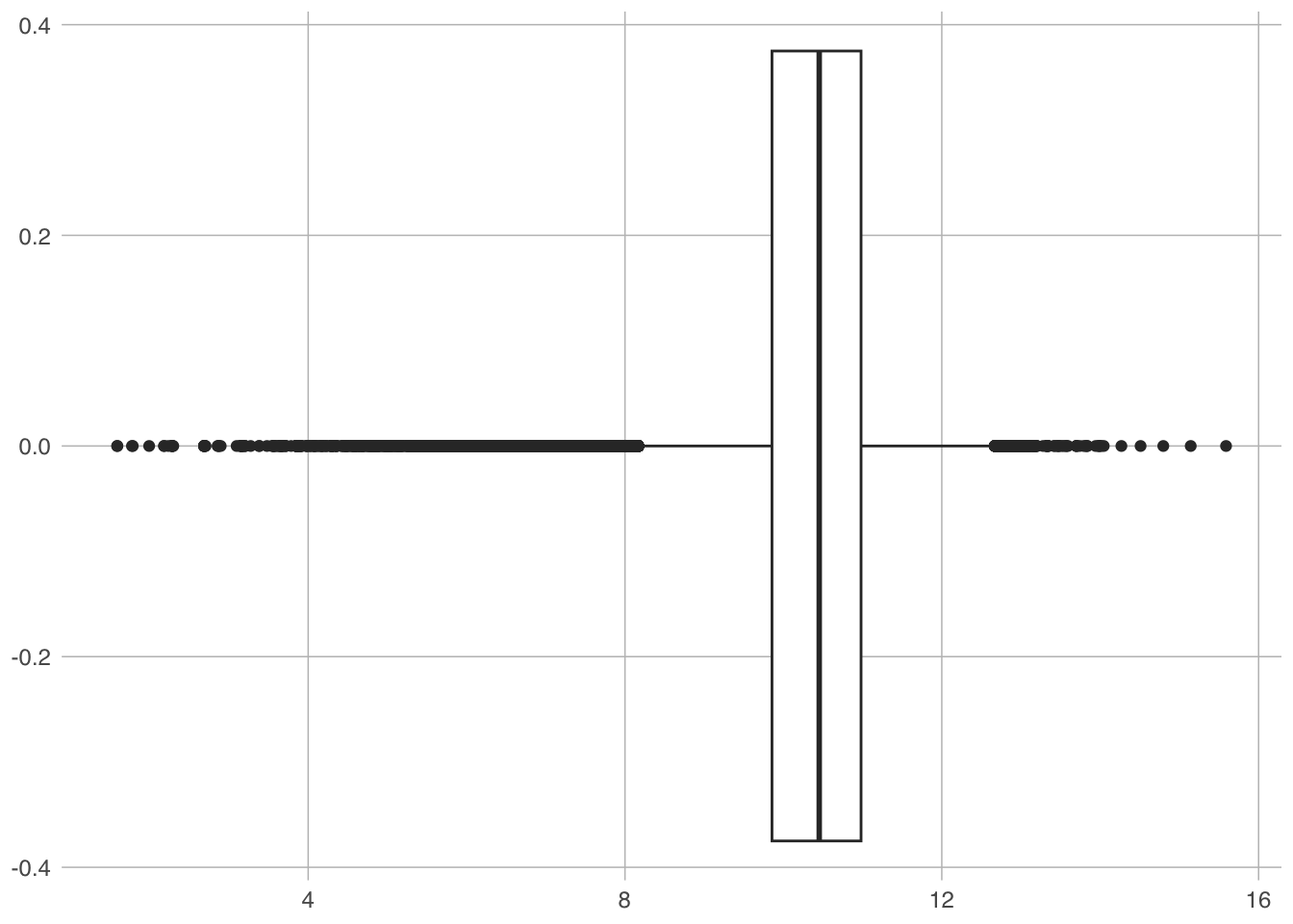
$ ingtrab <dbl> 35706.51, 66766.28, 93081.50, 0.00, 22255.43, 40255.41, 333…
$ trabajo <dbl> 35706.51, 66766.28, 51603.24, 0.00, 17364.13, 40255.41, 327…
$ sueldos <dbl> 33749.99, 61630.42, 41086.95, 0.00, 17364.13, 36586.94, 246…
$ horas_extr <dbl> 0.00, 0.00, 978.26, 0.00, 0.00, 0.00, 7092.39, 0.00, 0.00, …
$ comisiones <dbl> 0.00, 0.00, 0.00, 0.00, 0.00, 0.00, 0.00, 0.00, 0.00, 0.00,…
$ aguinaldo <dbl> 1956.52, 4646.73, 5135.86, 0.00, 0.00, 3668.47, 1027.17, 0.…
$ indemtrab <dbl> 0, 0, 0, 0, 0, 0, 0, 0, 0, 0, 0, 0, 0, 0, 0, 0, 0, 0, 0, 0,…
$ otra_rem <dbl> 0.00, 489.13, 4402.17, 0.00, 0.00, 0.00, 0.00, 0.00, 0.00, …
$ remu_espec <dbl> 0, 0, 0, 0, 0, 0, 0, 0, 0, 0, 0, 0, 0, 0, 0, 0, 0, 0, 0, 0,…
$ negocio <dbl> 0.00, 0.00, 41478.26, 0.00, 0.00, 0.00, 0.00, 0.00, 0.00, 0…
$ noagrop <dbl> 0.00, 0.00, 41478.26, 0.00, 0.00, 0.00, 0.00, 0.00, 0.00, 0…
$ industria <dbl> 0, 0, 0, 0, 0, 0, 0, 0, 0, 0, 0, 0, 0, 0, 0, 0, 0, 0, 0, 0,…
$ comercio <dbl> 0, 0, 0, 0, 0, 0, 0, 0, 0, 0, 0, 0, 0, 0, 0, 0, 0, 0, 0, 0,…
$ servicios <dbl> 0.00, 0.00, 41478.26, 0.00, 0.00, 0.00, 0.00, 0.00, 0.00, 0…
$ agrope <dbl> 0, 0, 0, 0, 0, 0, 0, 0, 0, 0, 0, 0, 0, 0, 0, 0, 0, 0, 0, 0,…
$ agricolas <dbl> 0, 0, 0, 0, 0, 0, 0, 0, 0, 0, 0, 0, 0, 0, 0, 0, 0, 0, 0, 0,…
$ pecuarios <dbl> 0, 0, 0, 0, 0, 0, 0, 0, 0, 0, 0, 0, 0, 0, 0, 0, 0, 0, 0, 0,…
$ reproducc <dbl> 0, 0, 0, 0, 0, 0, 0, 0, 0, 0, 0, 0, 0, 0, 0, 0, 0, 0, 0, 0,…
$ pesca <dbl> 0, 0, 0, 0, 0, 0, 0, 0, 0, 0, 0, 0, 0, 0, 0, 0, 0, 0, 0, 0,…
$ otros_trab <dbl> 0.00, 0.00, 0.00, 0.00, 4891.30, 0.00, 586.95, 0.00, 0.00, …
$ rentas <dbl> 0.00, 32282.60, 11739.13, 0.00, 0.00, 72684.78, 0.00, 0.00,…
$ utilidad <dbl> 0.00, 0.00, 0.00, 0.00, 0.00, 72684.78, 0.00, 0.00, 16007.2…
$ arrenda <dbl> 0.00, 32282.60, 11739.13, 0.00, 0.00, 0.00, 0.00, 0.00, 0.0…
$ transfer <dbl> 8804.34, 8999.99, 0.00, 90538.03, 1956.52, 0.00, 26902.17, …
$ jubilacion <dbl> 0.00, 0.00, 0.00, 79239.13, 0.00, 0.00, 0.00, 73369.56, 440…
$ becas <dbl> 391.3, 0.0, 0.0, 0.0, 0.0, 0.0, 0.0, 0.0, 0.0, 0.0, 0.0, 0.…
$ donativos <dbl> 0.00, 0.00, 0.00, 0.00, 1956.52, 0.00, 26902.17, 0.00, 0.00…
$ remesas <dbl> 978.26, 0.00, 0.00, 0.00, 0.00, 0.00, 0.00, 0.00, 0.00, 0.0…
$ bene_gob <dbl> 7434.78, 0.00, 0.00, 11298.90, 0.00, 0.00, 0.00, 5649.45, 0…
$ transf_hog <dbl> 0.00, 8999.99, 0.00, 0.00, 0.00, 0.00, 0.00, 2442.84, 0.00,…
$ trans_inst <dbl> 0, 0, 0, 0, 0, 0, 0, 0, 0, 0, 0, 0, 0, 0, 0, 0, 0, 0, 0, 0,…
$ estim_alqu <dbl> 11612.90, 0.00, 29032.25, 14516.12, 0.00, 8709.67, 0.00, 14…
$ otros_ing <dbl> 0, 0, 0, 0, 0, 0, 0, 0, 0, 0, 0, 0, 0, 0, 0, 0, 0, 0, 0, 0,…
$ gasto_mon <dbl> 35091.17, 78670.73, 101647.27, 46702.31, 26927.85, 51176.07…
$ alimentos <dbl> 9514.19, 17524.25, 18321.36, 14759.90, 12458.47, 6351.40, 1…
$ ali_dentro <dbl> 6814.20, 5181.41, 16907.08, 6274.20, 7315.63, 951.42, 11828…
$ cereales <dbl> 1465.70, 231.42, 1362.84, 1928.53, 308.56, 617.14, 1915.67,…
$ carnes <dbl> 617.14, 4114.28, 5142.85, 1928.57, 2442.84, 0.00, 6685.69, …
$ pescado <dbl> 0.00, 0.00, 0.00, 0.00, 1799.99, 0.00, 1414.28, 0.00, 0.00,…
$ leche <dbl> 269.99, 578.57, 0.00, 1414.26, 0.00, 334.28, 0.00, 565.70, …
$ huevo <dbl> 0.00, 257.14, 1028.57, 0.00, 321.42, 0.00, 0.00, 0.00, 1002…
$ aceites <dbl> 0.00, 0.00, 565.71, 0.00, 0.00, 0.00, 0.00, 0.00, 0.00, 0.0…
$ tuberculo <dbl> 0.00, 0.00, 0.00, 0.00, 1028.56, 0.00, 321.42, 621.38, 0.00…
$ verduras <dbl> 2288.53, 0.00, 1735.69, 1002.84, 642.85, 0.00, 951.41, 2069…
$ frutas <dbl> 1954.27, 0.00, 0.00, 0.00, 0.00, 0.00, 539.99, 1234.27, 195…
$ azucar <dbl> 0.00, 0.00, 0.00, 0.00, 0.00, 0.00, 0.00, 0.00, 0.00, 0.00,…
$ cafe <dbl> 0.00, 0.00, 0.00, 0.00, 0.00, 0.00, 0.00, 0.00, 0.00, 0.00,…
$ especias <dbl> 218.57, 0.00, 0.00, 0.00, 0.00, 0.00, 0.00, 0.00, 0.00, 0.0…
$ otros_alim <dbl> 0.00, 0.00, 5142.85, 0.00, 0.00, 0.00, 0.00, 3857.14, 1928.…
$ bebidas <dbl> 0.00, 0.00, 1928.57, 0.00, 771.41, 0.00, 0.00, 462.84, 2378…
$ ali_fuera <dbl> 2699.99, 12342.84, 1414.28, 8485.70, 5142.84, 5399.98, 5528…
$ tabaco <dbl> 0.00, 0.00, 0.00, 0.00, 0.00, 0.00, 0.00, 0.00, 0.00, 0.00,…
$ vesti_calz <dbl> 2445.64, 684.78, 0.00, 1369.56, 0.00, 1751.06, 9782.60, 489…
$ vestido <dbl> 2445.64, 684.78, 0.00, 1369.56, 0.00, 1751.06, 5380.43, 489…
$ calzado <dbl> 0.00, 0.00, 0.00, 0.00, 0.00, 0.00, 4402.17, 0.00, 0.00, 0.…
$ vivienda <dbl> 1736.75, 29649.66, 3232.25, 2850.00, 2700.00, 3660.00, 1822…
$ alquiler <dbl> 0.00, 24677.41, 0.00, 0.00, 0.00, 0.00, 13935.48, 0.00, 0.0…
$ pred_cons <dbl> 116.75, 2032.25, 2032.25, 150.00, 0.00, 150.00, 0.00, 750.0…
$ agua <dbl> 780, 540, 750, 450, 450, 1200, 1410, 420, 840, 420, 900, 87…
$ energia <dbl> 840.00, 2400.00, 450.00, 2250.00, 2250.00, 2310.00, 2876.61…
$ limpieza <dbl> 2075.80, 2816.11, 1422.55, 1228.04, 890.36, 3518.67, 2386.3…
$ cuidados <dbl> 2075.80, 2816.11, 1422.55, 1228.04, 792.54, 3518.67, 2386.3…
$ utensilios <dbl> 0.00, 0.00, 0.00, 0.00, 97.82, 0.00, 0.00, 0.00, 489.13, 23…
$ enseres <dbl> 0.00, 0.00, 0.00, 0.00, 0.00, 0.00, 0.00, 0.00, 0.00, 0.00,…
$ salud <dbl> 2641.29, 0.00, 0.00, 0.00, 0.00, 1007.60, 8902.16, 3277.16,…
$ atenc_ambu <dbl> 2641.29, 0.00, 0.00, 0.00, 0.00, 1007.60, 7923.90, 3277.16,…
$ hospital <dbl> 0.00, 0.00, 0.00, 0.00, 0.00, 0.00, 0.00, 0.00, 0.00, 0.00,…
$ medicinas <dbl> 0.00, 0.00, 0.00, 0.00, 0.00, 0.00, 978.26, 0.00, 978.26, 0…
$ transporte <dbl> 6773.62, 6706.44, 23312.90, 23574.19, 5080.63, 20601.28, 84…
$ publico <dbl> 2314.28, 0.00, 0.00, 0.00, 0.00, 0.00, 0.00, 771.42, 1157.1…
$ foraneo <dbl> 0, 0, 0, 0, 0, 0, 0, 0, 0, 0, 0, 0, 0, 0, 0, 0, 0, 0, 0, 0,…
$ adqui_vehi <dbl> 0, 0, 0, 0, 0, 0, 0, 0, 0, 0, 0, 0, 0, 0, 0, 0, 0, 0, 0, 0,…
$ mantenim <dbl> 2903.22, 4354.83, 11612.90, 20322.58, 4064.51, 17709.67, 53…
$ refaccion <dbl> 0, 0, 0, 0, 0, 0, 0, 0, 0, 0, 0, 0, 0, 0, 0, 0, 0, 0, 0, 0,…
$ combus <dbl> 2903.22, 4354.83, 11612.90, 20322.58, 4064.51, 17709.67, 53…
$ comunica <dbl> 1556.12, 2351.61, 11700.00, 3251.61, 1016.12, 2891.61, 3033…
$ educa_espa <dbl> 2903.22, 0.00, 34728.25, 0.00, 4209.66, 6967.74, 9058.05, 0…
$ educacion <dbl> 2903.22, 0.00, 0.00, 0.00, 0.00, 6967.74, 6735.47, 0.00, 0.…
$ esparci <dbl> 0.00, 0.00, 5380.43, 0.00, 4209.66, 0.00, 2322.58, 0.00, 0.…
$ paq_turist <dbl> 0.00, 0.00, 29347.82, 0.00, 0.00, 0.00, 0.00, 0.00, 0.00, 0…
$ personales <dbl> 4097.44, 3870.14, 13416.08, 2920.62, 1344.17, 812.90, 4918.…
$ cuida_pers <dbl> 673.53, 3745.14, 1916.09, 2920.62, 1344.17, 812.90, 4708.95…
$ acces_pers <dbl> 0.00, 0.00, 0.00, 0.00, 0.00, 0.00, 0.00, 0.00, 0.00, 0.00,…
$ otros_gas <dbl> 3423.91, 125.00, 11499.99, 0.00, 0.00, 0.00, 210.00, 0.00, …
$ transf_gas <dbl> 2903.22, 17419.35, 7213.88, 0.00, 244.56, 6505.42, 73.36, 4…
$ percep_tot <dbl> 0.00, 0.00, 0.00, 0.00, 3214.27, 0.00, 0.00, 0.00, 0.00, 0.…
$ retiro_inv <dbl> 0, 0, 0, 0, 0, 0, 0, 0, 0, 0, 0, 0, 0, 0, 0, 0, 0, 0, 0, 0,…
$ prestamos <dbl> 0, 0, 0, 0, 0, 0, 0, 0, 0, 0, 0, 0, 0, 0, 0, 0, 0, 0, 0, 0,…
$ otras_perc <dbl> 0, 0, 0, 0, 0, 0, 0, 0, 0, 0, 0, 0, 0, 0, 0, 0, 0, 0, 0, 0,…
$ ero_nm_viv <dbl> 0, 0, 0, 0, 0, 0, 0, 0, 0, 0, 0, 0, 0, 0, 0, 0, 0, 0, 0, 0,…
$ ero_nm_hog <dbl> 0.00, 0.00, 0.00, 0.00, 3214.27, 0.00, 0.00, 0.00, 0.00, 0.…
$ erogac_tot <dbl> 0.00, 19565.21, 0.00, 28124.99, 0.00, 5771.73, 360.97, 2445…
$ cuota_viv <dbl> 0, 0, 0, 0, 0, 0, 0, 0, 0, 0, 0, 0, 0, 0, 0, 0, 0, 0, 0, 0,…
$ mater_serv <dbl> 0.00, 0.00, 0.00, 0.00, 0.00, 0.00, 0.00, 0.00, 0.00, 0.00,…
$ material <dbl> 0, 0, 0, 0, 0, 0, 0, 0, 0, 0, 0, 0, 0, 0, 0, 0, 0, 0, 0, 0,…
$ servicio <dbl> 0.00, 0.00, 0.00, 0.00, 0.00, 0.00, 0.00, 0.00, 0.00, 0.00,…
$ deposito <dbl> 0.00, 19565.21, 0.00, 28124.99, 0.00, 5771.73, 0.00, 2445.6…
$ prest_terc <dbl> 0.00, 0.00, 0.00, 0.00, 0.00, 0.00, 0.00, 0.00, 0.00, 0.00,…
$ pago_tarje <dbl> 0.00, 0.00, 0.00, 0.00, 0.00, 0.00, 0.00, 0.00, 0.00, 0.00,…
$ deudas <dbl> 0.00, 0.00, 0.00, 0.00, 0.00, 0.00, 0.00, 0.00, 0.00, 0.00,…
$ balance <dbl> 0.00, 0.00, 0.00, 0.00, 0.00, 0.00, 0.00, 0.00, 0.00, 0.00,…
$ otras_erog <dbl> 0.00, 0.00, 0.00, 0.00, 0.00, 0.00, 360.97, 0.00, 0.00, 0.0…
$ smg <dbl> 15558.3, 15558.3, 15558.3, 15558.3, 15558.3, 15558.3, 15558…